MBC design problem

mbc design, Use mbc mfile to do problem I gave you in class i.e. study how plots change as you vary k and z in K = k [ (s+z)/s ] [ 1000/(s+1000) ]^2; P1 = (s-200)/(s-2) , P2 = (s-20)/(s-2) , and P3 = (s-4)/(s-2) Comment on sens and comp sens (Understand how a small rhp zero makes the control problem more challenging)

Contents

clc; clear; close all;

Form Plant P1=(s-200)/(s-2) P2=(s-20)/(s-2) P3=(s-4)/(s-2)

ap = 2; bp = -198; cp = 1; dp = 1;
plant1 = ss(ap,-198,cp,dp);
plant2 = ss(ap,-18,cp,dp);
plant3 = ss(ap,-2,cp,dp);

Using Plant 1 with k=-0.1 z=2

disp('Using Plant 1 with k=-0.1 z=2')
HW1_MBC(-0.1,2,plant1) % choose k, z, plant to use and call mfile

Using Plant 1 with k=-0.1 z=2
Open Loop Poles:
                                            
 Eigenvalue      Damping     Freq. (rad/s)  
                                            
  0.00e+000    -1.00e+000      0.00e+000    
  2.00e+000    -1.00e+000      2.00e+000    
 -1.00e+003     1.00e+000      1.00e+003    
 -1.00e+003     1.00e+000      1.00e+003    
                                            
ol_zeros =
  1.0e+002 *
  -0.02000000000000   2.00000000000000
Closed Loop Poles:
                                            
 Eigenvalue      Damping     Freq. (rad/s)  
                                            
 -2.58e+000     1.00e+000      2.58e+000    
 -1.81e+001     1.00e+000      1.81e+001    
 -6.39e+002     1.00e+000      6.39e+002    
 -1.34e+003     1.00e+000      1.34e+003    
                                            
sen_zeros =
  1.0e+003 *
   0.00200000000000  -1.00000000366348  -0.99999999633652   0.00000000000000

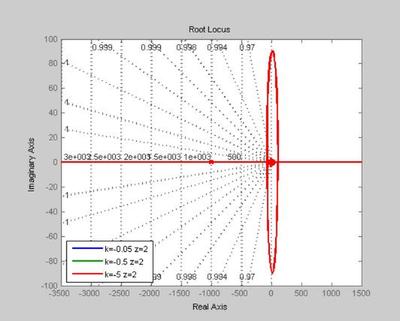
Using Plant 2 with k=-0.5 z=2

disp('Using Plant 2 with k=-0.5 z=2')
HW1_MBC(-0.5,2,plant2); % choose k, z, plant to use and call mfile

Using Plant 2 with k=-0.5 z=2
Open Loop Poles:
                                            
 Eigenvalue      Damping     Freq. (rad/s)  
                                            
  0.00e+000    -1.00e+000      0.00e+000    
  2.00e+000    -1.00e+000      2.00e+000    
 -1.00e+003     1.00e+000      1.00e+003    
 -1.00e+003     1.00e+000      1.00e+003    
                                            
ol_zeros =
    -2    20
Closed Loop Poles:
                                            
 Eigenvalue      Damping     Freq. (rad/s)  
                                            
 -3.94e+000     1.00e+000      3.94e+000    
 -1.09e+001     1.00e+000      1.09e+001    
 -2.73e+002     1.00e+000      2.73e+002    
 -1.71e+003     1.00e+000      1.71e+003    
                                            
sen_zeros =
  1.0e+002 *
  Columns 1 through 2 
  0.02000000000000                     -9.99999999999999 - 0.00000033722220i
  Columns 3 through 4 
 -9.99999999999999 + 0.00000033722220i  0.00000000000000                    

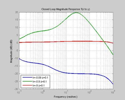
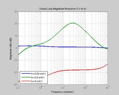
Using Plant 3 with k=-0.9 z=0.1

disp('Using Plant 3 with k=-0.9 z=0.1')
HW1_MBC(-0.9,0.1,plant3) % choose k, z, plant to use and call mfile

Using Plant 3 with k=-0.9 z=0.1
Open Loop Poles:
                                            
 Eigenvalue      Damping     Freq. (rad/s)  
                                            
  0.00e+000    -1.00e+000      0.00e+000    
  2.00e+000    -1.00e+000      2.00e+000    
 -1.00e+003     1.00e+000      1.00e+003    
 -1.00e+003     1.00e+000      1.00e+003    
                                            
ol_zeros =
  -0.10000000000000   4.00000000000000
Closed Loop Poles:
                                                         
        Eigenvalue            Damping     Freq. (rad/s)  
                                                         
 -2.42e-001                  1.00e+000      2.42e-001    
 -2.43e+001 + 1.31e+001i     8.80e-001      2.76e+001    
 -2.43e+001 - 1.31e+001i     8.80e-001      2.76e+001    
 -1.95e+003                  1.00e+000      1.95e+003    
                                                         
sen_zeros =
  1.0e+002 *
  Columns 1 through 2 
  0.02000000000000                     -9.99999999999999 - 0.00000016861110i
  Columns 3 through 4 
 -9.99999999999999 + 0.00000016861110i -0.00000000000000                    

Published with MATLAB® 7.1